File formats

File format list

The file formats currently supported by COPT are listed below:

Table 28 Supported file formats
Fileformat	File extension
MPS model file	`.mps`, `.mps.gz`
LP model file	`.lp`, `.lp.gz`
SDPA model file	`.dat-s`, `.dat-s.gz`
CBF model file	`.cbf`, `.cbf.gz`
model file in COPT binary format	`.bin`, `.bin.gz`
basis file	`.bas`
solution file	`.sol`
IIS file	`.iis`
FeasRelax file	`.relax`
MIP initial solution file	`.mst`
parameter file	`.par`
parameter tuning file	`.tune`

File I/O operations

By calling the relevant functions, users can input external model files to COPT for reading. At the same time, they can also save the output of the modeling and optimization results of COPT and output the files.

Let’s take reading/writing the model in MPS format in the current directory as an example (similar operations are performed for other files). The implementation methods in different interfaces are as follows:

Table 29 Functions for input and output files
API	Input	Output
COPT cmd	`read example.mps`	`write example.mps`
C	`COPT_ReadMps`	`COPT_WriteMps`
Python	`Model.read()` / `Model.readMps()`	`Model.write()` / `Model.writeMps()`
C++	`Model::read()` / `Model::readMps()`	`Model::write()` / `Model::writeMps()`
C#	`Model.Read()` / `Model.ReadMps()`	`Model.Write()` / `Model.WriteMps()`
Java	`Model.read()` / `Model.readMps()`	`Model.write()` / `Model.writeMps()`

Model file introduction

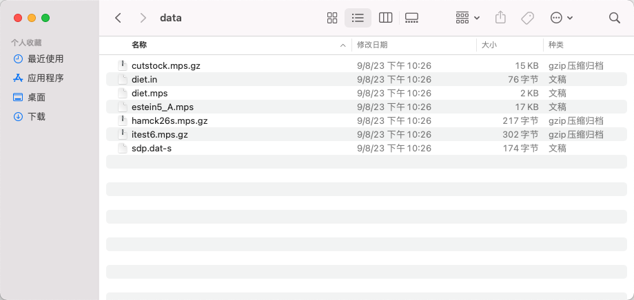
Users can find the model file examples that come with COPT in the "examples/data" directory of the installation package. Here we introduce the specific contents of two common model file formats: MPS and LP.

MPS format

MPS is a universal model file standard format. Different types of optimization problems can be output and stored in mps format, which is widely used in optimization softwares.

The following is an example of a model file in MPS format:

NAME          COPTPROB
OBJSENSE
    MAX
ROWS
N  __OBJ___
L  R0000000
G  R0000001
COLUMNS
    x         __OBJ___  1.2
    x         R0000000  1.5
    x         R0000001  0.80000000000000004
    y         __OBJ___  1.8
    y         R0000000  1.2
    y         R0000001  0.59999999999999998
    z         __OBJ___  2.1000000000000001
    z         R0000000  1.8
    z         R0000001  0.90000000000000002
RHS
    RHS       R0000000  2.6000000000000001
    RHS       R0000001  1.2
BOUNDS
LO BOUND     x         0.10000000000000001
UP BOUND     x         0.59999999999999998
LO BOUND     y         0.20000000000000001
UP BOUND     y         1.5
LO BOUND     z         0.29999999999999999
UP BOUND     z         2.7999999999999998
ENDATA

This MPS format example mainly includes several parts: NAME, OBJSENSE, ROWS, COLUMNS, RHS, and BOUNDS.

NAME: The name of the model
OBJSENSE: Optimization direction of the objective function
ROWS: Constraints and their directions in the model (L means <= constraints, G means >= constraints, N means no boundaries)
COLUMNS: Variables and their coefficients in the model
RHS: The value of the right-hand term of the constraint
BOUNDS: Bounds of variables (LO means lower bound, UP means upper bound, FR means no bounds)

Notes

In the ROWS section, the first line __OBJ___ represents the objective function.
In the COLS part, the form x __OBJ___ 1.2 indicates that the coefficient of variable x in the objective function is 1.2.
In MPS format, integer variables will be identified by the following fields:
- First integer variable: MARKER 'MARKER' 'INTORG'
- Last integer variable: MARKER 'MARKER' 'INTEND'

LP format

The LP format is closer to the algebraic form. It is more readable than MPS, and can easily correspond to its original mathematical model.

The following is an example of a model file in LP format:

\Generated by Cardinal Operations

Maximize
1.2 x + 1.8 y + 2.1 z
Subject To
1.5 x + 1.2 y + 1.8 z <= 2.6
0.8 x + 0.6 y + 0.9 z >= 1.2
Bounds
0.1 <= x <= 0.6
0.2 <= y <= 1.5
0.3 <= z <= 2.8
END

This LP format mainly includes several parts: objective function (Maximize), constraints (Subject To), and variable scope (Bounds).

Notes

In some LP format file, we can see variable names in the form x#1, which marks x as the first variable. When the user does not specify a variable name, this is the name automatically generated when outputting the lp model file.
If there is a binary type in the variable, it will be identified by the Binaries field.